An Obituary for the European Union
Extract from An introduction to European History Published 2050.
With hindsight, it appears obvious that the structure of the Greece bailout of 2010 was an error of catastrophic proportions. By partially socialising the losses of a banking system in crisis due to an impending sovereign default, European leaders transformed a banking and financial crisis into a contest between nations, unleashing titanic political forces which the Euro-zone’s unfinished political institutions could not hope to contain. Like the League of Nations before it, the Eurozone institutions depended on the large nations of Europe both to behave with restraint, and to enforce Commission directives on the smaller nations, since they were institutionally incapable of enforcing decisions when large countries violated commission directives.
The first warning signs cam in the pre-crises era, when France and Germany became serial violators of the Stability and Growth Pact. While punitive procedures were started against Portugal in 2002, and Greece in 2005, no such proceedings were initiated against either Germany or France, despite being serial violators. This inability to offer fair and equal treatment to all Euro-zone Members proved to be a serious contributory factor to the unfolding crisis.
Finally, perhaps the decisive factor, was the insularity and hubris of Europe’s Governing elite, who allowed their views to become divorced both from the public opinion in the countries they governed, and from economic reality. Indeed, in the crucial days of 2015, which now seem to be the chance to avert disintegration, Anglo-American economic commentators looked on in disbelief at creditor behaviour which would not have looked out of place among the debtor prisons of Victorian England.
The financial crisis of 2008-09 had myriad causes, but in the Eurozone two features stand out. Firstly, that European regulation gave to all European sovereign debt a risk weight of zero, which allowed banks to effectively up-risk their portfolios while staying within their capital limits, and indeed, this was an extremely profitable trade from 1999-2006, massively enriching bank shareholders as periphery interest rates declined towards the levels seen in core European Countries, and secondly, that there were large intra-country financial flows driven by different economic policies which encouraged some nations to run surpluses. Although the currency would adjust to counteract large surpluses at the level of the Euro-zone, there was no such balancing of intra-country flows inside the currency area, allowing Germany to build current account surpluses as periphery nations built large balancing deficits. Indeed, in some sense these flows of capital were a success of the European project, allowing capital to flow to those countries who most needed it. As it turned out, the financial infrastructure of periphery nations was simply not well enough developed to ensure that this money was channelled into efficient investment. Instead much went to finance consumption. In fact, given the scale of the inflows, it is extremely unlikely that any country could absorb capital flows of this magnitude relative to GDP. A historical parallel will be discussed below.
It is striking to note how little scope periphery nations had to prevent this build up of debt. Spain and Greek engaged in opposite policies. Spain ran a large government surplus, of which the end result was only to drive the cheap loans from the core into private sector debt via a boom in housing construction and financing. Greece ran persistent public sector deficits to absorb this capital flow, which resulted in having private sector debts which were among the smallest in the Eurozone. According to Eurostat private sector greek debt rose from 41% in 1998 to 93% in 2006. Spain, by comparison, grew its private sector debt from 89% to 193%. Germany and Austria, by way of comparison, saw private debt remain stable at around 120% of GDP.
This, then, was the Hobson’s choice presented to periphery countries by Euro membership: run a large government deficit or allow a dangerous level of growth in private debt, with the implicit associations of malinvestment and bubbles. This was a predicament that the German’s might have had sympathy with. Indeed, history is replete with parallels where dramatic capital inflows lead to enormous bubbles in financial assets. Perhaps the most notable was that in Germany following its victory of the Franco-Prussian war of 1871. Germany received an “indemnity” of around 20% of German GDP (5 billion gold frans) over three years. By driving the German current account into massive deficit, and a deficit being by definition an excess of investment over savings, the end result was a speculative mania culminating in a massive stock market boom in 1873 and a crash which it took years to recover from. Micheal Pettis’s article is an absolutely vital primer for anyone wishing to understand how these balance of payment issues drove the European debt crisis. The French economy, on the other hand, went from strength to strength, to the extent that by 1873 Germany was considering returning part or all of the indemnity!
The main point to understand then, is that the periphery had very little control over the build up of debt in their countries, two solutions were available (1) policies that increased Germanic consumption, and reduced their terms of trade advantage by raising wages. (2) A vast and well organised infrastructure spending campaign on behalf of the periphery, which was sufficiently productivity enhancing so as to support their worsening terms of trade.
The second option is a pipe dream, any country with a bureaucratic infrastructure which could design and implement such a program would already be a rich country which already had the financial infrastructure to handle large capital flows. Even some very successful countries lack the kind of institutional capital needed to organise such a program: The US and the UK stand out for having very poor infrastructure given their overall levels of development. The first option was of the table for political reasons, as in the Germanic view, being an exporter with a large current account surplus was a sign of success to be emulated. Never mind that such emulation was impossible, as the sum of intra-country surplus and deficits must be the deficit between the EZ and the world, and the Euro would adjust to keep that relatively close to zero. Thus, for Germany to run a persistent surplus inside the EZ, it was necessary for other countries to run persistent deficits.
This sets the stage for the crisis which was to prove the EZ’s undoing, however, it should be noted that the rate of convergence between the periphery and the core was truly startling, and given another twenty years of relative stability in the global economy, these imbalances may have worked themselves out. However, fate intervened, and the Global Financial Crisis of 2008 threw the solvency of almost every major European Bank into doubt. At this point. Capital flows reversed and even went into reverse as investors rushed to the safety of Core bonds. With investment spending collapsing, unemployment and budget deficits exploded around the periphery just as spreads widened and the reality that a EZ sovereign might default dawned on financial markets, further damaging confidence in the banks.
Greece in particular found financing its deficits difficult, and in 2010 asked for and received a bailout. The standard template for sovereign default has long since been settled on by the IMF. You first restructure the debt, while offering bridging finance to allow the affected party to meet their obligations until they regain market access. In return you get a program of reforms designed to enhance competitiveness. The Greek bailout did not follow this template. The exact reasons are unclear (as the Eurogroup does not publish minutes we shall probably never know), but the basic premise can be surmised: Greek debt was mainly held by European banks, which were already feared to be insolvent. Restructuring Greek debt might lead to panic in the financial markets.
This was a justifiable concern, however, the template for rescuing banks is even more settled than that of rescuing sovereigns. You simply inject capital directly into the affected financial institutions using the balance sheet of your central bank. You receive in return an equity stake. If even more capital is needed you wipe out the bondholders at the same time. Indeed, had the Eurozone followed this template, much, if not all, of the subsequent politics might have been obviated. We can only speculate about the true motives of those involved, but there was certainly an element of hubris. Jean-Claude Trichet, then president of the ECB, demanded that there should be no haircut, perhaps worried about financial contagion.
At this point the IMF was in deep conflict with its Eurogroup partners, as the IMF’s own rules demanded restructuring, and there was little or no way that Greece’s debts could be deemed sustainable without restructuring. These conflicting demands where “made consistent” by the assumption of wildly optimistic growth forecasts. Thus the first bailout agreed to swap existing Greek debt at par for official loans with gentler profiles, amounting to a small reduction in face value. It should be seen then that from the outset this was at least partially, and possibly mostly, a bailout of European Financial Institutions, rather than the Greek people, with some estimates suggesting that more than 2/3 of the headline figure of the bailout was an implicit gift to the financial intuitions which held Greek debt.
However, this narrative was never publicly expressed, it was rather dressed up as a the generosity of the core towards the feckless Greeks who, despite an inability to manage their own affairs, where still fellow Europeans. This narrative allowed a poisonous dynamic to take place in public discourse, as the program failed to deliver its promised growth projections, and a second and third bailout was needed, it appeared that Greeks were just chronically unable to manage their finances, and that Greek was a black hole for the European Tax payer. Indeed, now that most Greek liabilities were held by the public it was much harder to manage debt re-profiling as that would be a direct loss to the European taxpayer, and a possible violation of the Lisbon treaty’s prohibition on financing Eurozone Governments. By this stage the economics were firmly in the back seat to the political considerations. In 2015 Greece elected a new government with a mandate to renegotiate the bailout. Greece’s primary concern was to get debt relief and restructuring in return for further reforms. In other words, that the Eurogroup should admit that they made a mistake in their original bailout, and should eat their losses by reducing the face value of greek debt. Politically, this was impossible for the Eurozone, however much economic sense it made. It was at this stage that it first became clear to the author the enormous difference between the Anglo-American view of debt and what we might term the “Teutonic view”.
In the Anglo-American view when one buys a bond one purchases, among other things, the default risk. This risk was the primary differentiator of European government bonds, which faced identical inflation and duration risks as members of a single currency area. When purchasing such a bond one trusts that the issuer will make a good faith effort to repay you, but you also accept, that in the event of unforeseen circumstances, the issuer has the unilateral right to restructure your bonds so as to maximise utility. There will be a cost for this in terms of future market interest rates, or in the case of default on institutions like the IMF in terms of future aid. But the issuer has the unilateral right to decide to default either partially or totally if they think the costs are less than the benefits. To my mind, the Eurogroup, in their first and second bailouts had effectively bought the default risk of Greece, which would materialise if, and only if, their economic projections turned out to be optimistic. This indeed is a sensible economic perspective, which aligns the incentives for debtor and creditor in a similar way to Chapter 11 Bankruptcy in the US. If the creditor wants to be made whole, he must support actions which maximise the value of his claims, which could only be fulfilled if the Greek economy was growing. This was a view shared by many commentators. The “Teutonic View”, held most obviously by Wolfgang Schauble, was that Greece had a moral duty to repay its creditors in full whatever the cost. The fact that the creditors toxic mix of austerity had all but destroyed Greek’s economy, or that the original bailout’s success was predicated on forecasts which turned out to be wildly optimistic, was of no consequence. Greece was to make good its creditors and its only recourse was to abandon the Euro and accept the immense pain that would inevitably follow.
No where was this made more clear than in the Eurogroup summit of 2015:
Firstly, the Eurogroup rejected all responsibility for the failure of its program of austerity, instead claiming:
There are serious concerns regarding the sustainability of Greek debt. This is due to the easing of policies during the last twelve months, which resulted in the recent deterioration in the domestic macroeconomic and financial environment. The Eurogroup recalls that the euro area Member States have, throughout the last few years, adopted a remarkable set of measures supporting Greece’s debt sustainability, which have smoothened Greece’s debt servicing path and reduced costs significantly.
This runs so completely contrary to established economic wisdom that it is difficult to see any virtue in this statement other than a desire to further strengthen the political narrative that the creditors are blameless, have only acted selflessly to aid Greece, and have been stymied by the failure of the Greek establishment to fully implement their totally reasonable “solutions”.
The Eurogroup stresses that [nominal] haircuts on the debt cannot be undertaken.
The Greek authorities reiterate their unequivocal commitment to honour their financial obligations to all their creditors fully and timely.
I.e. complete acceptance of the “Teutonic view” that the creditors bear no responsibility for the failure of the program that they designed, and no acceptance that the original bailout program had any other aims than the salvation of the Greek people from their “carefree” and “populist” government.
Moreover, it is obvious in retrospect that the creditor governments were setting Greece up for an impossible situations. With Greece’s economy imploding there was zero chance that supply sire reforms would have any impact, and may actually make things worse in the short term. One must also ask, with historical detachment why, if the implementation of the OECD toolkits was so vital to Greece “regaining competitiveness” its implementation was not asked for in earlier bailouts? If the measures were not sufficient in 2010, is the ever more rigorous commitment to reform not a comment on the earlier failed programs? At any rate, it is well established that reforms of the supply side will have little or no affect while the demand side of the economy is depressed. Increasing potential growth will have little effect on an economy already far from potential and rapidly deterioration. The economic reality is that Greece needs stimulus. Fiscal multipliers were certainly large in Greece, given its inordinately large unemployment, in such cases stimulus lowers debt burdens and austerity increases them.
Thus, in 2015 the Eurogroup committed Greece to another failed bailout and another trip round the merry-go-round of ever increasing debt burdens and falling national income which rapidly made the new forecasts as obsolete as the old ones.
At this point a mention should be made of the ECB. It was at this stage that the true political divisions of the ECB were revealed. A true central bank, faced with a locally imploding economy, would act swiftly and promptly to intervene to support the banking system. Instead it acted to deliberately cap Emergency lending, so that Greece was forced to issue capital controls to prevent the complete collapse of its system. This move further destabilised the Greek economy, which was, if not recovering, at least flirting with an exit to recession. This revealed that the ECB was not an independent central bank intent on fulfilling its mandate, but a political entity controlled by the northern Europeans. The rate rise in 2011 and failure to do QE was subsequently recast as more than an error of judgement, but instead a deliberate attempt to favour Germany and the core. After all, a robust recovery would have rebalanced German wages through moderate inflation and wage increases, leading to lower balance of payments problems. It was now clear that an unelected and unaccountable body was not independent and was instead the enforcer for a group of unaccountable finance ministers who kept no minutes of their meetings and operated with a total lack of transparency.
The outrage among the twittering classes was instant and enormous. For a dry euro-group statement to engender such open hostility from all sides was a shock, as the #ThisIsACoup gained traction in almost all European countries it quickly became clear that any who thought making an example out of Greece would quell support for populist parties had miscalculated badly. What they failed to see was the subsequent realignment of European Domestic Politics. European integration was The Issue. It was no longer left vs right, or socialist vs free market, or even ordoliberal vs statist. It was now pro-integration or pro-repatriation. The previously stable centre ground of a quiet drift towards more power for European Institutions came to an abrupt halt. Trust in the benevolence of Franco-German leadership evaporated as quickly as Hollande rounded on Merkel for putting Grexit on the table. The IMF and former US treasury secretary Tim Geithner’s accounts of Eurogroup discourse became must reads for all those who styled themselves as “intelligentsia”, and they made for damning reading. Geithner described the Eurogroup as early as 2010 as “wanting to take a bat to Greece”. Sarkozy and Merkel asked president Obama to help them force out Berlusconi, a democratically elected leader of a major European economy.
We can get a sense of the outrage across Europe by looking at some of the commentary:
Wolfgang Munchau, an influential FT commentator, said:
A few things that many of us took for granted, and that some of us believed in, ended in a single weekend. By forcing Alexis Tsipras into a humiliating defeat, Greece’s creditors have done a lot more than bring about regime change in Greece or endanger its relations with the eurozone. They have destroyed the eurozone as we know it and demolished the idea of a monetary union as a step towards a democratic political union.
Paul Krugman, Nobel Prize winner and NY Times columnist:
Even if all of that is true, this Eurogroup list of demands is madness. The trending hashtag ThisIsACoup is exactly right. This goes beyond harsh into pure vindictiveness, complete destruction of national sovereignty, and no hope of relief. It is, presumably, meant to be an offer Greece can’t accept; but even so, it’s a grotesque betrayal of everything the European project was supposed to stand for.
European democracies might have been pre-occupied by the immediate after affects of the crisis, but by the time the Third Greek Bailout had dissolved into acrimony as the Greek economy imploded there was no more room for inaction. Greece didn’t come asking for a fourth bailout. They just closed their banks in December 2015 and announced they were re-denominating. Having retained control of their assets they wiped out all their creditors with a total default. And the worst part for the Germans was, the private creditors didn’t mind at all. Greece got market access almost at once and its recovery, following six months of pain, was dramatic. Redenomination risk was back for all European Sovereigns. Spain and Ireland were by this stage recovering rapidly, but the election of governments extremely sceptical of the European project meant that the UK was no longer a lone voice calling for the repatriation of powers. From the point of view of the European Institutions, this only made it all the more vital that none be surrendered. Within the wider economic union the division grew wider. With Poland and Ireland wishing to exempt themselves from the legalisation of Euthanasia across Europe in late 2016, they traded the promise of a British veto for support for the renegotiation of British membership. In the event the British, along with most of the non-euro states agree to exit the European Union but to stay part of the common market, and to have a say in shaping common market policy. With the British exit from the European Union, the dream of a unified Europe died.
Without that dream, the Germans became increasingly unsettled about paying for a Europe which offered them little, and which included an increasingly embittered relationship with the French. In the end the Euro dissolved. Germany, Austria Belgium, the Netherlands, Finland and Luxembourg remained within the rump of the euro, along with most of the minor states. Spain and Portugal and France started a new currency. Italy and Cyprus went their own way.
The European Union became little more than than a common market, of little practical importance as a political entity, although still a useful forum for European Powers to negotiate trade agreements and economic agreements.
Evidence for the slope of the supply curve
This is a companion post to the previous one. In that post I argued that NGDP was superior when the supply curve is nearly flat, in this one I argue that the empirical evidence strongly favours a flat supply curve at the following times.
What follows are a series of plots of RGDP vs NGDP with associated trend lines.

We are looking at the slope of the supply curve.
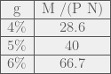
The gradient of this graph is 0.55, it shows a reasonable correlation of 
Now lets look at 1990-Present, i.e. the era of low inflation. Now we see:

This shows RGDP vs NGDP 1990-Present
Note that now, in this era, a 1% point rise in NGDP is associated with a 0.85% rise in RGDP. I.e. The supply curve is very flat. This is exactly the danger area identified in my previous post, where in order to reduce inflation by a small amount, one must sacrifice a huge amount of output. A 1% reduction in inflation would correspond to a 6% reduction in output. Note also that the correlation is a lot better in this era, than in the whole data set. This should increase our confidence that this is a meaningful subset – i.e. that there is something qualitative different about this selection of points from a random sampling. In this case, the adoption of a low inflation target.
We can also estimate “expected inflation” from this analysis. Expected inflation is the level of NGDP growth needed for RGDP to be flat, so in this case, 1.44/0.849 = 1.7%. Since this is close to the inflation target, that is further evidence that this analysis is meaningful.
Lets look at the 1970’s. We might expect that this is a time when we got onto the vertical part of the supply curve, :

Note that even in this era, the supply curve appears flat, it just has an enormous intercept.
This time we have an expected inflation reading of 6.5%, along side an almost identical gradient. We can say here with some confidence that inflation expectations were higher in the 1970’s, but what to make of the identical gradient? I expect what we are seeing here is expectation adjustment. Every time the expectations adjust you get moved back onto the flatter part of the supply curve. This is the theory of the inflation adjusted Philips curve. This causes the correlation to break down, as a change in inflation expectation moves the whole line up and down.
Lets look at this era in more detail:

This shows how inflation expectations developed
Here are two periods, Oct 68 to Jan 72, and Oct 73-79/01. In both of these periods we get pretty good correlations, but inflation expectations have jumped, and the supply curve becomes even flatter. Perhaps what is happening here is that as uncertainty about inflation becomes chronic, output falls, and we get onto the flatter part of the supply curve. Here inflation expectations jumped 5 percentage points in a few years. This is indeed puzzling. Perhaps the real lesson here is that the supply/demand framework does not work well without a nominal anchor around which to have “unexpected” stimulus.
Nevertheless, the broad point stands: Throughout the 1990’s, the trade off between inflation and output was terrible. Thus, attempts to keep inflation on target by tightening policy in response to a 1% supply side shock to prices, would result in around a 6% loss of output. Given the small costs of small deviations from the inflation target, central banks should be prepared to tolerate deviations from the inflation target, provided that they are doing so in order to keep aggregate demand more stable, because the costs of a loss of demand are huge, and the costs of missing your inflation target are tiny.
Nowhere is this more clear than in the 2011 rate tightening of the European Central bank, which in order to prevent a small overrun in its inflation target, was forced to induce a catastrophic loss of demand.
Visualising NGDP Targeting
The AS-AS framework gave rise to one of the iconic images of Economics. Almost everyone who has studied or followed economics will have seen a version of the following diagram:

The AS-AD Diagram – from Wikimedia commons
Now, the stylised facts of this diagram are these
- The supply curve is upward sloping : A higher price usually means a larger quantity can be produced. Think of how a higher price of Oil makes hard to reach reservoirs economic.
- The supply curve goes vertical at some finite level of output. This represents real constraints on production in the economy.
- The demand curve is downwards sloping – generally people buy a larger quantity of stuff when its cheaper.
We can understand the inflation targeting regime through the lens of this diagram. A supply shock moves the supply curve upwards. In order to return to the target price level, the central bank must move the demand curve leftwards. This is the reason to believe that inflation targeting is a sub-optimal strategy for a central bank – in this framework, in response to a positive supply shock, which decreases output, a central bank must deliberately generate a further fall in output in order to get inflation back to target. Think about that – in order to keep inflation on target in the face of a supply shock, we must deliberated produce less than we could. Moreover, in the real world, a loss of demand almost always means a rise in unemployment. So we are deliberately trading unemployment and lost production for in order to hit a 2% target.
The reverse happens in a positive supply shock. This time the supply curve is lowered, so the central bank shifts the AD curve rightwards. This rise in demand leads to a boom, and when the supply shock passes we find that the aggregate demand curve is too far to the right (policy is suddenly too loose) and we get a spike in inflation.
In the real world, its fair to say that we don’t “know” the shape of the supply curve and the aggregate demand curve. All we can measure is the cross over which actually happens i.e., we can measure the price level and RGDP and Lets specify aggregate demand by: 


This diagram is just the AS-AD diagram with a third axis drawn on to represent NGDP. The red lines are lines of constant NGDP. The inspiration for this was Minkowski diagrams for switching between space time frames by drawing on the a second frame of reference.
A supply shock hits the economy, and as a result the supply curve moves from A to B. Originally, this moves us from the point marked start, to the point marked NGDP. Under NGDP targeting, this is where the story ends, as we have moved along a line of constant NGDP. We have some slightly higher inflation, and a small decrease in output, but this output loss was inevitable, as the new supply curve goes vertical well below the original level of output. Under inflation targeting, the central bank now forces AD/NGDP onto a lower path, inorder to return the price level to its starting value, Pi. This cause output to drop from Yn to Yi. In the example that I have drawn, where the supply curve is fairly flat, the decrease in output needed to bring inflation back to its starting value was far larger than the original loss of output. This is the disaster scenario for inflation targeting, where a large loss of output is required to correct a small change in inflation. This is arguably what happened in the US in 2008, and almost certainly what happened to the Eurozone in 2011, where policy makers focused on inflation, traded catastrophic falls in output to a void small overruns in inflation.
Of course, if I had moved the start point up onto the nearly vertical part of the supply curve, then we could have traded a tiny loss in output for quite a large change in the price level. Arguably, this was the story of the 70;s and 80s, where they were in a reasonably high inflation regime, and this put them well onto the vertical part of the supply curve, this, huge changes in inflation translated into only small changes in output.
On more nice thing about this diagram: it makes it clear that what we actually have are two `real’ things, the supply curve, and the demand curve. But these are unmeasurable, and we can specify the outcomes (where the curves cross) using any two of NGDP, real output, and the price level. The price level/Real output specification seems to have an almost sacred place in economics. When given a choice of equivalent decompositions, it is almost always right to thing in terms of the things which are easiest to measure. Here that ist he Price Level, and NGDP. An independent measurement of real output is almost impossible, as it would depend on some kind of notion of intrinsic value, so in practice, RGDP is measured by applying an inflation correction to NGDP. By using a Y,P decomposition, you are cross-correlating your measurement errors.
Finally, NGDP targeting always leads to a smaller output gap but higher inflation than IT when faced with a supply shock. If we are on the flat part of the supply curve, that is a good thing, if we are on the vertical part of the supply shock, that is a bad thing. given the general downards stickiness of inflation despite enormous falls in output in the US, UK, and EZ, we are definitely on the flat part of the curve, and so should be looking to NGDP growth, rather than inflation, to guide policy.
Deflation, Coming to a Continent near you
Deflation has finally arrived in Europe. It is now undeniably hear. While Mario Draghi continues to claim that inflation expectations are well anchored, the reality is that the ECB has waited too long to act, and now has a mountain to climb. They have repeated the policy mistakes of the Fed in the 1930s or Japan in the 1990’s, and refused to believe that monetary policy was the correct tool to manage aggregate demand. I am, in all honesty, surprised by the length of time it has taken. Ever since the ECB raised rates in 2011, choking off a nascent recovery this has been the predictable outcome. I thought 12% unemployment in the Eurozone would drive deflation in 2012. I suspect this is a feature of how we measure inflation. I have a whole series of posts coming up on how to measure inflation better, based on my original foray into this space, and some musings of the Atlanta Fed’s statistician, plus some Machine Learning insights.
Anyway, I just wanted to chronicle the arrival of deflation today:
The CPI recorded an annual rate of change of -0.9% in July 2014. Excluding energy and unprocessed food, the annual rate was -0.4%. The CPI monthly rate decreased to -0.7% (0.1% in June 2014 and -0.2% in July 2013), while the CPI 12-month average rate was -0.2% in July.

The EU-harmonised index (HICP):
                             JULY        JUNE         MAY
 Monthly change              -2.1         0.1        -0.1
 Yr/yr inflation              0.0         0.2         0.4
 Index (base 2005=100)      117.9       120.4       120.3

The NIC index:
 Monthly change              -0.1         0.1        -0.1
 Yr-on-yr inflation           0.1         0.3         0.5
 Index (base 2010=100)      107.5       107.6       107.5


Of course, Greece:

and Cyprus:

Even Sweden:

But don’t worry, this is all a needed competitive adjustment, which we can see directly from the robust inflation rates in the other, stronger UK economies:

Or perhaps from the robust inflation in the Eurozone as a whole?

Deflation is here. The ECB is out of excuses, and out of time. If it cannot deploy QE because of political impediments, then this depression is about to get worse. A lot worse. Ill leave you with some comments from a market economist, via Joe Weithensal:
For Euroland, the big picture is that the economy is in its seventh year of depression. On our estimate of a 0.7% contraction in the second quarter, GDP was still 3.2% lower than it was in the first quarter of 2008, when the depression began. Euroland’s economy actually contracted in the first quarter of this year when you exclude Germany’s unexpected surge to a 3.3% annualized rate of growth. Only people who were misled by Markit’s untested and unproven PMIs believed that such growth was real and sustainable. Our estimate of second quarter GDP for the Euro Zone includes a contraction of Germany’s economy at a 2% annualized rate, reversing the windfall in the unexplained and inexplicable first quarter spurt. If our forecast proves correct, average GDP growth for Germany in the first half of 2014 will work out to 0.7% at an annualized rate, clearly less than potential but very much in line with the experience over the last few years. Our estimate for France’s economy is a more horrible contraction of 1.1% for the quarter, or 4.3% at an annualized rate.
Italy’s Recovery

I saw this graphic referenced on Twitter.
Just incredible to see that five years into the Eurozone “recover” Italy is not only below its pre-crisis peak, its below its post crisis trough. Even more amazing to see how the ECB’s rate rise in 2011 choked off the nascent Italian recovery.
There is an ECB rate meeting today, since the last one inflation has fallen to just 0.4%, and inflation expectations have also fallen. I wonder what excuse Draghi will come up with this time to not announce QE.
Programming, Life Lessons, and the Power of Forgetfulness
This post is somewhat whimisical, and is spaned by a fascinating article that I read on REgular Expression Pattern matching over at swtch.com .
Regular Expressions are a way of categorising strings of letters and symbols so that you can have a powerful tool for searching text for strings of a particular form, or for insisting that they come in a particular form. For example, you could search a block of text and pull our every set of 7 characters which could be a UK number plate.
Anyway, it turns out that there is an extremely efficient algorithm for doing this matching known as Thompson NFA. This algorithm has been known since almost the beginning of RegEx. It was implemented in early Linux Kernals from the 1970’s. It turns out, that almost no modern language implements this algorithm, instead, they use much much worse versions in their common library functions. How much worse? Well, for a 100 character string Thomson NFA takes 200 microseconds, while Perl would require 10^15 years.
The performance graph is here:

Sorry What? A powerful, fast and efficient algorithm has been known for years, yet most modern programming languages use a vastly inferior version. Why?
It turns out, that communities just forget things. RegEx became what JH Newman called “furniture of the mind”, a concept that you are comfortable with, but don’t really need to understand. When writing their libraries, RegEx functions are just things like maths functions, you implement them because every language should ahve them, but you don’t pay too much attention to them. They are just the boring bricks and mortar of programming.
So Pery, Ruby, Python and Java all shipped with a RegEx algorithm orders of magnitude worse than the best one, and often with more code needed to implement this badly.
Scott Sumner has a theory that Central banks are always fighting the last war, as their domain knowledge is formed when you are studying in your twenties and thirties. People who grew up in the 1970’s are obsessed with inflation. People who grew up in the 1930s were obsessed with deflation. Here is that dynamic in a totally context. Those CS graduates who grew up with RegEx was an interesting and open problem in the 50s and 60s knew about the best algorithms, and implemented in the languages and operating systems of that era. Then it was done, and everyone just used it without understanding it, and the knowledge was `lost’. The next generation created exciting object orientated paradigms and just forgot that this was once an interesting problem with an optimal solution, and just “did the obvious thing”, which turned out to be slow. Then they tried to improve it with a variety of clever tricks like memoisation, but none of that got over the inherent inferiority of the backtracking approach to RegEx matching.
How Much do NGDP expectations matter to the Stock Market?
The inspiration for this post was a brief discussion with a friend, when I attempted to explain why I think of the stock market as a prediction market for NGDP. We might pose the following question, if NGDP expectations were to increase from 5% per year to 6% per year for every year from now to forever, how much would that matter to the stock market?
The short answer is, a lot.
To answer this, lets take a slightly round about route of asking, what is the Net Present Value ,

There is some evidence that we might expect it to be at the higher end of this range going forward due to having more tech with higher profit margins, and more overseas earnings. So lets assume that this is stable at 


Where we have 
Given the assumptions above, if we assume that everything grows at a stable growth rate (i.e we are ignoring possible path dependency), then
So a 1% increase in NGDP gives about a 40% increase in the stock market, as a handy rule of thumb. No wonder the stock market loves QE!
If we take the EMH seriously, we must conclude that the combination of low TIPS spreads predicting low inflation, and a booming stock market predicting high NGDP, means that we can expect productivity/RGDP to come roaring back any minute now. A market Monetarist argument for Supply Side Optimism. Yes, I’m looking at You Britmouse. 🙂
What is happening in the Bond Market?
Across the developed markets, long bond yields are moving lower. Lower long yields typically represent lower expectations of NGDP. After all, if NGDP is expected to grow robustly, then either it will cause inflation and bonds will get killed, or it there will be high productivity growth, and stocks will likely do better.
Lower NGDP expectations must mean tighter policy in the short term. At least in my world view that is more or less the definition of tighter policy. Thus, when I see long bond yields move lower, I immediately ask, “who is tightening policy?”.
The answer seems to be everyone. China’s central bank is hard to read, but it appears happy to accept some level of slowdown to put a lid on rampant credit growth. The US is tapering, and good economic data out of Japan is causing people to rethink their expectations of the BOJ easing further. Finally, no one really thinks that the ECB will have the political will to do the kind of Japan level QE that the EZ desperately needs.
Now, despite all that, I don’t think that that is the primary driver of what is happening. I think that falling inflation in the short term (less than 2 years), has resulted in a passive tightening of policy, and that is what is crushing long yields. The real short term rate is the nominal bank rate (in the UK 0.5%) less inflation (annual change GDP deflator). The following graph therefore gives a sense of the “real” short term rate in the US.

So its pretty clear that the low inflation in the US has caused policy to tighten by almost a full percentage point since 2012. If you were to make an adjustment to this for the taper the effective tightening would be even greater. Sadly, I could not make the usually excellent Fred give me up to date series for the EZ GDP deflator – for some reason it ends in mid 2013. I strongly suspect the EZ is in an even worse position.
I think financial markets are waking up to the fact that low inflation might be here for a while, and that this has significant implications on where the “real” policy rate lies, even if there is no change in the expected path of the nominal rates. Remember, policy is expansionary *if and only if* the (real) natural short term interest rate is above the inflation adjusted Fed funds rate. Might we just have seen these cross over? If so, expect the US slowdown to continue, and Europe to go back over the cliff.
BOE’s Inflation Report
So I had a look at the FT’s coverage of the inflation report, and it brought up one of my pet peeves about the commentary on the crisis, namely, measures of economic slack.
The bank of England apparently thinks that there is around 1.5% of slack in the economy. My first pet hate is that “slack” is not adequately defined in this context. Does this mean that Carney thinks that RGDP will develop a new trend line that is only 1.5% higher than the current level and at around 2% a year? Or does this simply mean that at the current moment companies estimate that with their current personnel and facilities they could only increase production by 1.5%.
This is important because there are two types of “slack”, there is the measure of “could we do more right now”, and there is the measure “given greater demand could I deploy more employees, capital, and technology to increase supply”. I am pretty sure the BOE’s estimate is about the former, but the macroeconomically important version is the latter. In other words, the supply side constraints could be soft for a while, if technological improvements since 2008 have enabled greater production, but they just haven’t been deployed due to weak demand.
Lets take a quick look at the RGDP (constant prices):

Does this look like an economy with only 1.5% slack? Is it not possible that in the medium term we might recover nearly all of our lost productivity? Might we not find that as demand grows aggregate supply just continues to quietly grow so that the BOE’s measure remains stuck at 1.5% while GDP grows 4-5% a year for a number of years?

Stolen from an ONS publication, does this look like an economy with only 1.5% slack? Are you telling me that after 7 years of technological progress, the BOE expects slack in GDP to be exhausted before productivity per worker has even reached its 2007 high?
Are we really to expect that some (minor) institutional differences will mean that UK workers will not, over the medium term, enjoy the same advances that have allowed US productivity to grow 20% in the same period? The UK is structurally similar to the US, but the structural differences (might) mean that in the UK we get more hiring first, and productivity growth later, and in the US they get more productivity first, and then more hiring. That certainly seems more plausible to me than that the differences in our institutions mean that the UK will not benefit from the same advances of the US in the long run. In that case, the technology exists already for a 20% rise in productivity in UK workers.
The real problem here is that the BOE is giving a short term definition of slack, where it doesn’t assume anything about the future investment and employment and capital improvement programs of enterprises. It just asks about capacity utilisation right now. Which, immediately following a recession, is a sensible enough thing to do. The problem is, that here we have moved into the medium term. There has been technological progress in that time, and the fact that this is waiting in the wings means that we should not regard current utilisation as in anyway a meaningful indicator of “slack”.
I predict that productivity per worker will recover its century long trend line of 2% a year growth. In that case, “slack” in the economy is more like 15% than 1.5%. Capital spending, training workers on new technology, the rise of robotics and machine learning will do the heavy lifting over the next 3-5 years, and we can expect strong growth along side benign inflation until we approach this productivity trend line.
There is Still No Housing Bubble
Articles about Housing Bubbles are ten a penny at the moment, so I thought it was about time for another salvo in my lonely war against the Bubble Obsessed. When I was lying awake last night, it occurred to me that there is not really enough thought about what constitutes “expensive” or “cheap” when it comes to housing. When talking about an item like bread, we can see that over time the price tends to fall slowly as technology and farming improves, but with occasional spikes when there is some type of supply shock which lowers supply. So it makes sense to talk about when bread is expensive by comparing it to recent history. Fashion items, on the other hand, derive part of their value from their exclusivity, so their price relative to wages stays fairly constant to target a given type of consumer.
Then there are financial assets like the stock market, which make new highs most years, because they are a claim on a fraction of a pie which is growing. Since the housing market also a claim on future earnings, via rent, it too should logically make new highs most years.
It is my contention that housing is more of a luxury good than a commodity, and thus I would expect people to have a reasonably stable preference about what fraction of their income they are prepared to spend on housing. Thus, house prices are expensive, only in so far as they grow more than the total spending (perhaps per capita) in an economy. This makes sense, if my wages grow over time, I would expect to try to move to a better house, and pay more rent. Since, on average, everyone’s wages grow over time, so must house prices. Running to stand still as it were.
The following shows the change in the house price index relative first to NGDP (=total spending), and secondly to the median wage.

Look how stable house prices/median wages have been!!!
The first thing to note is how amazingly stable both these measures are over time. Particularly house prices/median wages. It was basically flat for decades. On the housing/nominal spending measure, US housing has never been cheaper! The difference in trajectory is a measure of the fact that median wages have not risen in line with total spending due to declining labour share over the period. It is interesting that prices relative to median wages really did show a marked increase in the 2000s, but that is all but fully unwound, and I look forward to watching house prices going flat relative to median wages for many more decades.
I tried to recreate the same graph for the UK, but FRED seems to only have rental income. However, that is interesting in its own right, so lets look at rental prices vs NGDP and vs the median wage in the UK:

Where is that house price bubble again?
This data goes over a much shorter period than the US data above. However, its pretty clear that the cost of renting has been in a reasonably long term decline throughout the nineties. I look forward to watching the cost of renting resume its decade long decline.
Its also interesting that the crash has actually made housing more expensive since it caused wages to fall much faster than house prices. A salutory warning to the Bundesbank and Swedish who seem determined to make the case that you should try to put a lid on house prices by raising rates.
Anyway, the main point is clear – forget the media’s obsession. Housing is cheap by the most important measure – its cost relative to median wages.
Also, if you are a BOE Hawk determined to raise rates to put the break on the housing market, then have another look at the evidence. And then don’t.
PS:If someone can find the data for UK house prices in a handy format somewhere, I will redo the US graph for the UK.
